Critical Value Calculator

What is a Critical Value?

A critical value is a cutoff point in a statistical test that separates the rejection region from the non-rejection region. Researchers, data analysts, and scientists use it to determine whether to reject the null hypothesis in hypothesis testing.

When you run a statistical test, you're asking: "Is this result significant enough to reject my null hypothesis?" The critical value answers that question. If your test statistic exceeds the critical value, you reject the null hypothesis. If it doesn't, you fail to reject it.

Critical values appear in medical research (testing new treatments), quality control (manufacturing standards), social sciences (survey analysis), business analytics (A/B testing), and scientific experiments. They're the threshold that determines whether your findings are statistically significant or just random noise.

Normal distribution curve showing two-tailed critical values at ±1.96 with 2.5% shaded area in each tail and 95% acceptance region in center

Distribution Types

Distribution	Best For	Required Info
Z-distribution	Large samples (n > 30) or known variance	α level, tail type
t-distribution	Small samples (n < 30), unknown variance	α level, df, tail type
Chi-square (χ²)	Variance tests, goodness-of-fit	α level, df, tail type
F-distribution	ANOVA, comparing two variances	α level, df&sub1;, df&sub2;, tail type
Pearson r	Correlation significance testing	α level, sample size, tail type

The critical value changes based on your chosen significance level (α), usually 0.05 or 0.01. A smaller α means you're being more conservative and requiring stronger evidence. The type of test (one-tailed vs. two-tailed) also affects the critical value. Two-tailed tests split α between both tails of the distribution, while one-tailed tests place it all in one direction.

How to Use the Critical Value Calculator

Using our critical value calculator is straightforward. Follow these steps to calculate critical values for any statistical test. You'll get instant results as you enter your parameters.

What You Need Before You Start

Test Type

Know if you need one-tailed or two-tailed test

Significance Level

Typically α = 0.05 or 0.01

Sample Info

Sample size (for df calculation)

Step-by-Step Guide

1
Choose your distribution - Select from Z, t, χ², F, or r. Use Z for large samples (n > 30), t for small samples, χ² for variance tests, F for ANOVA, and r for correlation tests.
2
Select test type - Pick two-tailed if you're testing for any difference (H₁: μ ≠ μ₀). Choose right-tailed if testing for increases (H₁: μ > μ₀) or left-tailed for decreases (H₁: μ < μ₀).
3
Enter significance level (α) - Most studies use 0.05 (5% error rate). Use 0.01 for stricter criteria or 0.10 for exploratory research. You can click quick buttons or type a custom value.
4
Add degrees of freedom (if needed) - For t and χ² tests, enter df = n - 1. For F-tests, enter both numerator (df₁) and denominator (df₂) degrees of freedom. For Pearson r, enter df = n - 2.
5
View your results - The critical value calculator displays your cutoff value instantly. For two-tailed tests, you'll see both lower and upper critical values.

Pro Tips for Accurate Results

Double-check your degrees of freedom calculation. For a sample of 25 in a t-test, df = 24 (n - 1).
Match your tail type to your hypothesis. If you're testing "is there a difference?" (not directional), use two-tailed.
Use the quick alpha buttons (0.01, 0.05, 0.10) for standard significance levels instead of typing.
For F-tests, don't confuse numerator and denominator df. Numerator comes from the between-groups variation.

How to Calculate Critical Values

To calculate critical values, you need to find the probability cutoff point for your chosen significance level. Here's the complete process for each distribution type.

The 4-Step Process to Calculate Critical Values

Choose your distribution

Based on sample size, known/unknown variance, and test type (mean, variance, correlation, or ANOVA).

Determine your significance level (α)

Common values: 0.05 (5%), 0.01 (1%), or 0.10 (10%). This represents acceptable Type I error rate.

Calculate degrees of freedom (if needed)

For t-tests: df = n - 1. For Chi-square: varies by test. For F-tests: df₁ and df₂ required.

Find the inverse CDF value

Use tables, statistical software, or our calculator to find the critical value at your specified probability level.

Manual Calculation vs. Critical Value Calculator

❌ Manual Calculation Challenges:

•Requires statistical tables (often limited precision)
•Time-consuming lookups and interpolation
•Risk of reading wrong row/column
•Limited to standard α values (0.05, 0.01)
•Complex inverse CDF calculations

✅ Using Critical Value Calculator:

•Instant results with high precision (4+ decimals)
•Works with any α value (custom inputs)
•No interpolation or table lookups needed
•Automatic tail-type adjustments
•Handles all distributions in one place

Z Critical Values

Z critical values come from the standard normal distribution (mean = 0, standard deviation = 1). Use Z critical values when your sample size is large (n ≥ 30) or when the population standard deviation is known.

Z Distribution Formula:

f(z) = \frac{1}{\sqrt{2\pi}} e^{-\frac{z^2}{2}}

Critical value: $z_\alpha$ where $P(Z > z_\alpha) = \alpha$

Common Z Critical Values:

• α = 0.05 (two-tailed): $\pm 1.96$
• α = 0.05 (one-tailed): $1.645$
• α = 0.01 (two-tailed): $\pm 2.576$
• α = 0.01 (one-tailed): $2.326$

t Critical Values

t critical values come from Student's t-distribution. Use t critical values when your sample size is small (n < 30) and the population standard deviation is unknown. The t-distribution has heavier tails than the normal distribution.

t Distribution Formula:

f(t) = \frac{\Gamma(\frac{\nu+1}{2})}{\sqrt{\nu\pi}\Gamma(\frac{\nu}{2})} \left(1 + \frac{t^2}{\nu}\right)^{-\frac{\nu+1}{2}}

Where $\nu$ = degrees of freedom (df = n - 1)

t Critical Values Examples (df = 20):

• α = 0.05 (two-tailed): $\pm 2.086$
• α = 0.05 (one-tailed): $1.725$
• α = 0.01 (two-tailed): $\pm 2.845$
• α = 0.01 (one-tailed): $2.528$

Chi-Square Critical Values

Chi-square critical values come from the chi-square distribution. Use chi-square critical values for variance tests, goodness-of-fit tests, and independence tests in contingency tables. Chi-square is always positive and right-skewed.

Chi-Square Distribution Formula:

f(x) = \frac{1}{2^{k/2}\Gamma(k/2)} x^{k/2-1} e^{-x/2}

Where k = degrees of freedom

Chi-Square Critical Values Examples (df = 10):

• α = 0.05 (right-tailed): $18.307$
• α = 0.05 (left-tailed): $3.940$
• α = 0.01 (right-tailed): $23.209$
• α = 0.01 (left-tailed): $2.558$

F Critical Values

F critical values come from the F-distribution. Use F critical values for ANOVA tests, comparing variances between groups, and regression analysis. The F-distribution requires two degrees of freedom: df₁ (numerator) and df₂ (denominator).

F Distribution Formula:

f(x) = \frac{\sqrt{\frac{(d_1x)^{d_1}d_2^{d_2}}{(d_1x+d_2)^{d_1+d_2}}}}{x \cdot B(d_1/2, d_2/2)}

Where $d_1$ = numerator df, $d_2$ = denominator df

F Critical Values Examples (df₁ = 5, df₂ = 20):

• α = 0.05 (right-tailed): $2.711$
• α = 0.05 (left-tailed): $0.311$
• α = 0.01 (right-tailed): $4.103$
• α = 0.01 (left-tailed): $0.164$

r Critical Values (Pearson Correlation)

Pearson r critical values are used for correlation tests. Use r critical values when testing whether a correlation coefficient is significantly different from zero. The critical value depends on sample size (n) and significance level.

Pearson Correlation Formula:

r = \frac{\sum(x_i - \bar{x})(y_i - \bar{y})}{\sqrt{\sum(x_i - \bar{x})^2 \sum(y_i - \bar{y})^2}}

Test statistic: $t = r\sqrt{\frac{n-2}{1-r^2}}$ follows t-distribution with df = n - 2

r Critical Values Examples (n = 30, df = 28):

• α = 0.05 (two-tailed): $\pm 0.361$
• α = 0.05 (one-tailed): $0.306$
• α = 0.01 (two-tailed): $\pm 0.463$
• α = 0.01 (one-tailed): $0.418$

Critical Value Formulas for All Distributions

Critical values come from probability distributions. Each distribution has a specific formula for finding the cutoff point that leaves exactly α probability in the tail(s). Below are the critical value formulas for Z, t, Chi-square, F, and Pearson r distributions.

Quick Reference: Critical Value Formulas

Z-Distribution

Two-tailed: z = Z⁻¹(1 - α/2)

Right-tailed: z = Z⁻¹(1 - α)

Left-tailed: z = Z⁻¹(α)

t-Distribution

Two-tailed: t = t⁻¹(1 - α/2, df)

Right-tailed: t = t⁻¹(1 - α, df)

Left-tailed: t = t⁻¹(α, df)

Chi-Square

χ² = χ²⁻¹(1 - α, df)

Most commonly right-tailed

F-Distribution

F = F⁻¹(1 - α, df₁, df₂)

Requires two df values

Important: The inverse CDF function (⁻¹) converts probability to the critical value. Our calculator computes these automatically.

Z-Distribution (Standard Normal)

For a two-tailed test with α = 0.05, we need the Z-value where 2.5% falls in each tail. The formula uses the inverse of the cumulative distribution function (CDF):

Two-tailed: z = Z^-1(1 - α/2)

Right-tailed: z = Z^-1(1 - α)

Left-tailed: z = Z^-1(α)

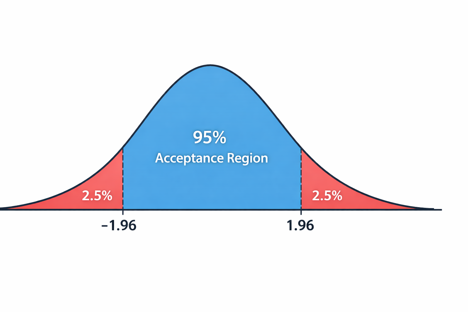
Example 1: Two-tailed test, α = 0.05

We want 95% in the middle, 2.5% in each tail.

Upper: z = Z^-1(1 - 0.025) = Z^-1(0.975) = 1.96

Lower: z = -1.96 (by symmetry)

This is the famous "±1.96" used in 95% confidence intervals. If your test statistic is below -1.96 or above 1.96, you reject H₀.

Example 2: Right-tailed test, α = 0.01

We want 99% to the left, 1% in the right tail.

z = Z^-1(0.99) = 2.33

This stricter cutoff means you need stronger evidence. Only the top 1% of values exceed 2.33.

t-Distribution

The t-distribution has heavier tails than the normal distribution. Critical values depend on degrees of freedom (df = n - 1):

Two-tailed: t = t^-1(1 - α/2, df)

Right-tailed: t = t^-1(1 - α, df)

Left-tailed: t = t^-1(α, df)

Example: Right-tailed test, α = 0.05, df = 18

Sample size n = 19, so df = 18

t = t^-1(0.95, 18) = 1.734

Notice this is smaller than the Z-value of 1.645 for the same α. Smaller samples need less extreme values due to wider distributions.

Edge case: Very large df (df = 100)

Two-tailed test, α = 0.05

t = t^-1(0.975, 100) ≈ 1.984

As df increases, t-values approach Z-values. At df = 100, we're very close to 1.96.

Chi-Square (χ²) Distribution

Chi-square tests are typically right-tailed. The distribution is always positive and right-skewed:

Right-tailed: χ² = χ²^-1(1 - α, df)

Example: Goodness-of-fit test, α = 0.05, df = 4

Testing if observed frequencies match expected

χ² = χ²^-1(0.95, 4) = 9.488

If your calculated χ² statistic exceeds 9.488, the differences between observed and expected are too large to be random chance.

F-Distribution

F-tests compare variances and require two degrees of freedom: numerator (df₁) and denominator (df₂):

Right-tailed: F = F^-1(1 - α, df₁, df₂)

Example: ANOVA test, α = 0.05, df₁ = 2, df₂ = 15

Comparing means of 3 groups (k=3), total n=18

df₁ = k - 1 = 2, df₂ = n - k = 15

F = F^-1(0.95, 2, 15) = 3.682

If your F-statistic is greater than 3.682, at least one group mean differs significantly from the others.

Remember: These calculations use inverse CDF functions, which are complex mathematical operations. Our calculator handles all the computation automatically, giving you accurate critical values instantly without manual lookup tables.

How to Interpret Critical Values in Hypothesis Testing

Once you have your critical value, compare it to your test statistic. The decision rule is simple: if your test statistic falls in the rejection region, you reject the null hypothesis.

Understanding Your Results

Two-tailed test

You get two critical values (lower and upper). Reject H₀ if your test statistic is less than the lower value or greater than the upper value. For example, with critical values of ±1.96, reject if your test statistic is below -1.96 or above 1.96.

Right-tailed test

You get one critical value. Reject H₀ if your test statistic is greater than this value. For example, with a critical value of 1.645, reject if your test statistic exceeds 1.645.

Left-tailed test

You get one critical value (negative). Reject H₀ if your test statistic is less than this value. For example, with a critical value of -1.645, reject if your test statistic is below -1.645.

What Factors Affect Critical Values?

1. Significance level (α)

Smaller α = larger critical values. Using α = 0.01 instead of 0.05 makes the critical value more extreme, requiring stronger evidence to reject H₀.

2. Tail type

Two-tailed tests split α between both tails, making each critical value slightly less extreme than one-tailed tests with the same α.

3. Degrees of freedom

For t, χ², and F distributions, fewer degrees of freedom = more extreme critical values (wider distributions need larger cutoffs).

4. Distribution type

Z-values are usually smallest, t-values slightly larger for small samples, χ² and F-values can be much larger depending on df.

5. Sample size (indirectly)

Larger samples mean more degrees of freedom, which brings critical values closer to the limiting distribution (t approaches Z as n increases).

6. Variance assumption

Known variance allows Z-tests. Unknown variance requires t-tests, which have larger critical values for small samples.

Critical Values vs P-Values vs Confidence Intervals

Critical values are part of a broader hypothesis testing framework. Here's how they relate to other statistical concepts.

Concept	Best For	Key Difference
Critical Values	Classical hypothesis testing with fixed α	Set cutoff before collecting data
P-values	Reporting exact probability of results	Shows strength of evidence, not binary decision
Confidence Intervals	Estimating population parameters with uncertainty	Provides range of plausible values, not just yes/no
Effect Sizes	Measuring practical significance	Shows magnitude of difference, not just existence
Bayesian Credible Intervals	Incorporating prior knowledge	Uses probability of hypothesis, not just data

When to use p-values instead:

P-values give you more information than a binary "reject/don't reject" decision. Use them when you want to show how strong your evidence is.

For example, p = 0.001 is much stronger evidence than p = 0.049, even though both are below α = 0.05.

When to use confidence intervals:

Confidence intervals show the range of plausible values for your parameter. They're more informative than hypothesis tests alone.

A 95% CI of [2.1, 5.8] tells you the effect is positive and gives you its likely magnitude.

When effect sizes matter more:

Statistical significance doesn't mean practical importance. A difference of 0.01% might be "significant" with 1 million samples but meaningless in practice.

Always report Cohen's d, eta-squared, or other effect size measures alongside significance tests.

Modern statistical reporting:

Many journals now require reporting confidence intervals, effect sizes, and exact p-values rather than just "p < 0.05."

This gives readers more information to judge the strength and importance of your findings.

Critical Value Calculator: Frequently Asked Questions

What's the difference between one-tailed and two-tailed critical values?

Two-tailed tests look for differences in either direction, so they split α between both tails. One-tailed tests put all α in one tail, making the critical value less extreme. For example, at α = 0.05, a two-tailed Z-test uses ±1.96, while a one-tailed test uses 1.645. Two-tailed tests are common in AB testing when you want to detect changes in either direction.

How do I know which distribution to use in my critical value calculator?

Use Z if your sample is large (n > 30) or you know the population variance. Use t for small samples with unknown variance. Use χ² for variance tests or goodness-of-fit. Use F for ANOVA or comparing two variances. Use r for testing correlation coefficients. When in doubt, t-tests are safer for small samples.

Why is my result different from a statistical table?

Statistical tables round values and may use different precision levels. Our calculator uses the exact inverse CDF formulas to compute critical values to 4 decimal places, which is more accurate than printed tables. Small differences (like 1.96 vs. 1.9600) are normal and don't affect conclusions.

Can I use this calculator for multiple comparisons?

Yes, but you need to adjust your α level first. If you're running 10 tests, divide your desired α by 10 (Bonferroni correction). For example, if you want overall α = 0.05 with 10 tests, use α = 0.005 for each test. Enter 0.005 in the calculator to get the adjusted critical value.

What's a good significance level (α) to use?

The standard is α = 0.05 (5% error rate), used in about 85% of studies. Use α = 0.01 for situations requiring stronger evidence (medical decisions, high-stakes research). Use α = 0.10 for exploratory research where false negatives are more costly than false positives. Don't adjust α after seeing your results.

How do degrees of freedom affect my critical value?

Lower degrees of freedom make the distribution wider, so critical values become more extreme. For a t-test with df = 5 and α = 0.05 (two-tailed), the critical value is ±2.571. With df = 30, it drops to ±2.042. As df increases above 100, t-values approach Z-values (±1.96 at α = 0.05).

Is a critical value the same as a confidence interval?

No, but they're related. Critical values determine the boundaries of hypothesis tests. Confidence intervals use critical values to create ranges around estimates. For example, a 95% CI uses the critical value of 1.96 (for Z) to calculate the interval as: estimate ± 1.96 × standard error.

What if my test statistic exactly equals the critical value?

By convention, you reject the null hypothesis if the test statistic equals or exceeds the critical value. However, borderline cases deserve extra scrutiny. Consider reporting the exact p-value, checking your assumptions, increasing sample size, or consulting a statistician before making important decisions.

Calculator Inputs

Critical Value Results

What is a Critical Value?

Distribution Types

How to Use the Critical Value Calculator

What You Need Before You Start

Step-by-Step Guide

Pro Tips for Accurate Results

How to Calculate Critical Values

The 4-Step Process to Calculate Critical Values

Manual Calculation vs. Critical Value Calculator

Z Critical Values

t Critical Values

Chi-Square Critical Values

F Critical Values

r Critical Values (Pearson Correlation)

Critical Value Formulas for All Distributions

Quick Reference: Critical Value Formulas

Z-Distribution (Standard Normal)

t-Distribution

Chi-Square (χ²) Distribution

F-Distribution

How to Interpret Critical Values in Hypothesis Testing

Understanding Your Results

What Factors Affect Critical Values?

Critical Values vs P-Values vs Confidence Intervals

When to use p-values instead:

When to use confidence intervals:

When effect sizes matter more:

Modern statistical reporting:

Critical Value Calculator: Frequently Asked Questions

What's the difference between one-tailed and two-tailed critical values?

How do I know which distribution to use in my critical value calculator?

Why is my result different from a statistical table?

Can I use this calculator for multiple comparisons?

What's a good significance level (α) to use?

How do degrees of freedom affect my critical value?

Is a critical value the same as a confidence interval?

What if my test statistic exactly equals the critical value?